Here at Level, we love graph-based data: whether studying the interaction between key players in the venture ecosystem or analyzing technical contributions on Github, we have a variety of data that fundamentally captures entities and the myriad relationships between them. For those uninitiated to the world of graphs (also called networks), we need but two types of information to define a graph: a set of things and a concept of connections between those things. As an example, here is a graph that represents the seating arrangement in our New York City office:

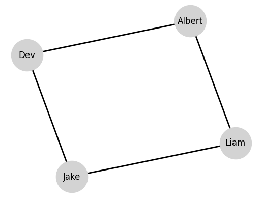
Of course, this example is a bit trivial. In the real world, graphs can be much more complex and interesting, and we mostly study dynamic graphs, where the connections between entities change over time. But we can use this opportunity to introduce important terminology: the entities in the graph are called nodes or vertices and the connections between them are called edges.

Graph Neural Networks

Everybody—even the Category Theorists—loves neural networks (themselves a type of graph) and we’re no different. So: given a set of graph-based data, how do we actually train a neural network to learn something about the underlying system? We’ll proceed by expositing a basic Graph Neural Network (GNN). Let’s imagine that we’re trying to predict the loudest person in the office (honestly, we already know it’s me). Where \(P\) is the set of people in the office, we can denote for each person \(i \in P\) a score \(x^{0}_{i}\) that represents their normal speaking volume in a quiet room by themselves. (That \(0\) in the superscript is just a way to denote the initial state of the system.)

How would you begin to model this problem? Well, it seems natural to assume that the loudness of a nearby person might influence the loudness of a person: after all, if I’m talking loudly to someone, we know that my interlocutor probably will also get louder to compensate. This is a classic example of a graph-based problem: the loudness of a person is influenced by the loudness of their neighbors. In fact, we use the term neighborhood to describe the set of nodes that are connected to a given node. For example, in the office graph above, the neighborhood of \(\text{Dev}\) is the set \(\{\text{Jake}, \text{Albert}\}\). In mathematical notation, we usually write the neighborhood of a node \(i\) as \(N_i\).

So, for a graph neural network, a layer takes in the current state of a node and its neighborhood and outputs a new state for the node. We can write

\[ x^{l}_i = f(x^{l - 1}_{i}, \overline{N}_{i}) \]

If we break the equation down: we say that we have a function \(f\) that accepts the previous loudness value of a node along with the loudness value of its neighbors and outputs a new loudness value for the node. The superscript \(l\) tells us which layer we are on: we start at \(l = 0\) (which is just our base data) and increment it as we go through the network. For the pedants, we define \(\overline{N}_{i} \triangleq \{x^{l - 1}_{j} \colon j \in N_{i}\}\) because we want to be clear that we are passing the loudness values of the neighbors (not the neighbors themselves) to the function \(f\).

Now, defining and learning \(f\) is the core of a GNN and there are a great variety of clever ways we can do this to train a neural network. We won’t explore those here, but a quick online search for GNNs will reveal a rich literature on the topic.

Graph Attention

We’ll refrain from making an [x] is all you need joke, but it’s true that attention has become a key concept in modern machine learning. Attention is a way of learning to focus on different parts of the input data and has been used to great effect in models like the Transformer: “Transformer” is the “T” in GPT. But attention as a mechanism is not limited to just natural language processing and can be applied to a variety of problems, including graphs.

V1

Now that we understand the general concept of a graph neural network, we can move on to a specific type of GNN called Graph Attention Networks (GAT), introduced in 2017 by Veličković, et al. In a GAT, we use a neural network to learn three parameters: a scalar value \(a_1\), a scalar value \(a_2\), and a scalar weight \(w\). We define a learned edge attention

\[ e_{i,j} \triangleq R(a_1 \cdot w x_{i} + a_2 \cdot w x_{j}) \]

where \(R\) is a non-linear activation function (traditionally LeakyReLU). (Note that we omit the superscript indicating the layer index where all terms are in the same layer.)

From here, we can define an attention coefficient for each edge:

\[ \alpha_{i, j} \triangleq \frac{\text{exp}(e_{i, j})}{\sum_{k \in N_{i}}\text{exp}(e_{i, k})} \]

All we’re doing here is re-scaling the edge attention values based on the neighborhood of a node, and in particular, we’re taking the softmax of the edge attention values over a node’s neighborhood.

Finally, we can write

\[ x^{l}_i = \sigma\left(\sum_{j \in N_{i}} \alpha^{l}_{i, j} \cdot w x^{l - 1}_{j}\right) \]

where \(\sigma\) is a non-linear activation function (traditionally LeakyReLU).

GATs are a great way of applying attention from models like a Transformer to the graph neural network context. However, it turns out that this version of GATs are not universal approximators and can’t learn all functions. Therefore, we need to introduce a more powerful version of GATs.

Dynamic Attention and V2

We won’t get into too many details of V2 (introduced in 2021 by Brody, et al.), but the main idea is to learn a dynamic attention mechanism (instead of a problematic static attention mechanism) that can learn to attend to different parts of the graph based on the input data. The change we make is just to redefine \(e\) as:

\[ e_{i,j} \triangleq a \cdot R(w_1 x_{i} + w_2 x_{j}) \]

It turns out that this formulation gives rise to a universal approximator. An interested reader can find more details in the original paper; note that the paper gives a more general formulation with vector-valued node features, but we provide a simplified real-valued version here for clarity.

This simple change is sufficient to go from a non-universal approximator to a universal approximator and, in particular, we can learn different attention weights for different parts of the graph based on the input data.

Dynamic Graphs and Attention

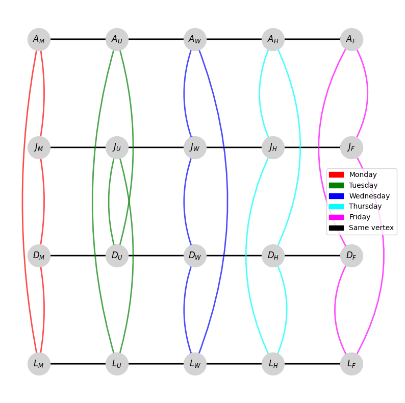
At Level, some of our most interesting datasets are dynamic graphs: the connections between entities change over time. In other words, instead of boring static edges, we have dynamic edges. Taking our earlier example of office seating, we might imagine a situation where we have “floating” desks: every day, we each take a different desk.

Let’s see how that would play out.

A Primer on Dynamic Graphs

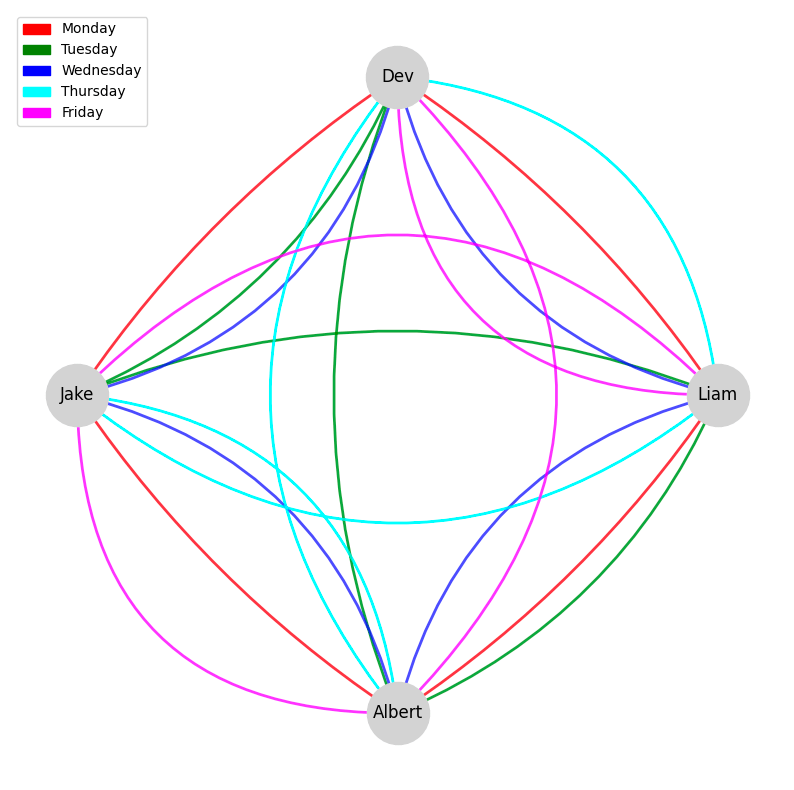
In the figure above, we can see the resulting dynamic network, where edges change over time. In this case, we have a seating chart that is changing every day: the different colors represent different days and the edges represent who sat next to whom on a given day. Another common strategy to represent such a dynamic network is a time-extended network, where we create multiple “copies” of each vertex over time. For example, we write \(A_M\) to represent Albert on Monday, \(J_U\) for Jake on Tuesday, \(L_H\) for Liam on Thursday, and so on. To actually generate the network, we have to connect the different copies of the same person over time, so we draw in edges following the direction of time for the same person.

One thing to keep in mind is that these graphs are not really “frozen” in time. Dynamic graphs are to movies as static graphs are to photographs: they capture a sequence of events and the relationships between entities change over time. Therefore, we would have to imagine this network changing over time in our heads; we can generate the above figures to help us visualize a dynamic network, but the actual network changes with respect to time.

Neural Networks + Dynamic Graphs = GAT V3

Now we connect both of our previous ideas: dynamic graphs and attention-based neural networks. One of the real datasets we use is a co-investment network: for a subset of fund managers, we track with whom they co-invest over time. This data naturally induces a dynamic network: every quarter, we draw an edge between two fund managers if they have an investment together. (It’s a bit more complicated than that, but we’ll leave it at this level of detail for now.)

With all of these components in mind, we can extend GAT V2 to dynamic graphs by learning dynamic attention in dynamic graphs. To do this, we use the representation of a dynamic network in Figure 2: a graph with multiple egdes between nodes representing information over time. (Formally, this structure is known as a multigraph.) We also update the attention mechanism to be:

\[ \begin{align*}{e'}_{i, j, t} &\triangleq a_{t} \cdot R(w_1 x_{i} + w_2 x_{j})\\ e_{i, j} &\triangleq \sum_{t, 't \in T} a'_{t, t'} {e'}_{i, j, t} \cdot {e'}_{i, j, t'}\end{align*} \]

Here, \(T\) represents all possible timesteps: therefore, we take the sum across time with time-based attention weights to compute our edge-based attention. (We leave out some technical details for clarity, e.g., handling edges that don’t exist at a given time.) With this mechanism, we actually compute spatiotemporal dynamic attention, which accounts for both spatial relationships (which nodes are in which neighborhood) and temporal relationships (how neighborhoods change over time).

We have additional architectural feature like special-handling of self-loops over time, inter-layer normalization, and multi-head attention, but we’ll leave those out for now. Again, it is also worth noting that we have vector-valued features; it is straightforward to carefully extend our real-valued features to vector-valued features.

Training Infrastructure and Testing Yoke

So, now that we have a model architecture and a relevant dataset, how do we actually run experiments? Our neural networks have decent number of hyperparameters in addition to their actual parameters (e.g. learning rate scheduling, number of layers, number of heads, etc.) and we need to run a large number of experiments to find the best model. In general, we use Weights & Biases (W&B) to track our various experiments. We then use a combination of quantitative and qualitative metrics to study and analyze how our models are performing.

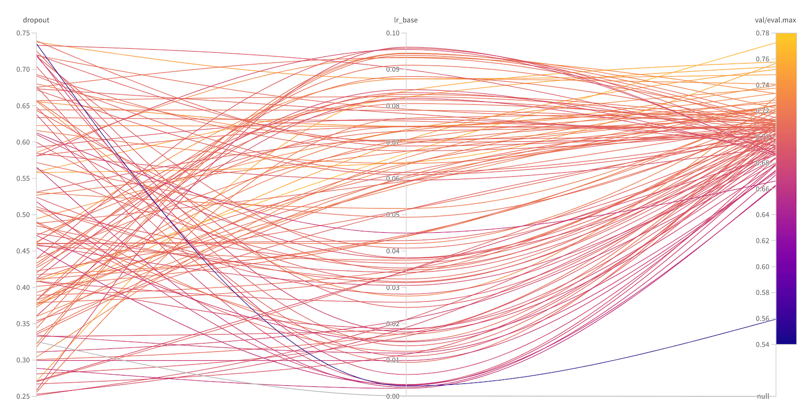
In terms of quantitative metrics, for each type of model, we try to develop a sensible loss, but also to design appropriate evaluation metrics that relate to the problem at hand: for example, one evaluation metric we might use is predicted firm performance of a known cohort of top-performing funds. Our loss function drives a single training instance, but our evaluation metrics typically drive early stopping and model selection. One common tactic we deploy is leveraging sweeps in W&B to run a large number of combinations of hyperparameters and we typically ask a sweep to optimize an evaluation metric, rather than the loss function. We have a variety of reasons for this, but the main one is that we often find that a sensible loss value does not correspond with the important metric for the task at hand. Loss functions have to be nice, differentiable, and efficient to compute, but evaluation metrics can be more complex, incorporate missing values, and so on. The figure below is a real sweep we ran for one of our core models that was trying to select best model based on a dropout rate and a base learning rate.

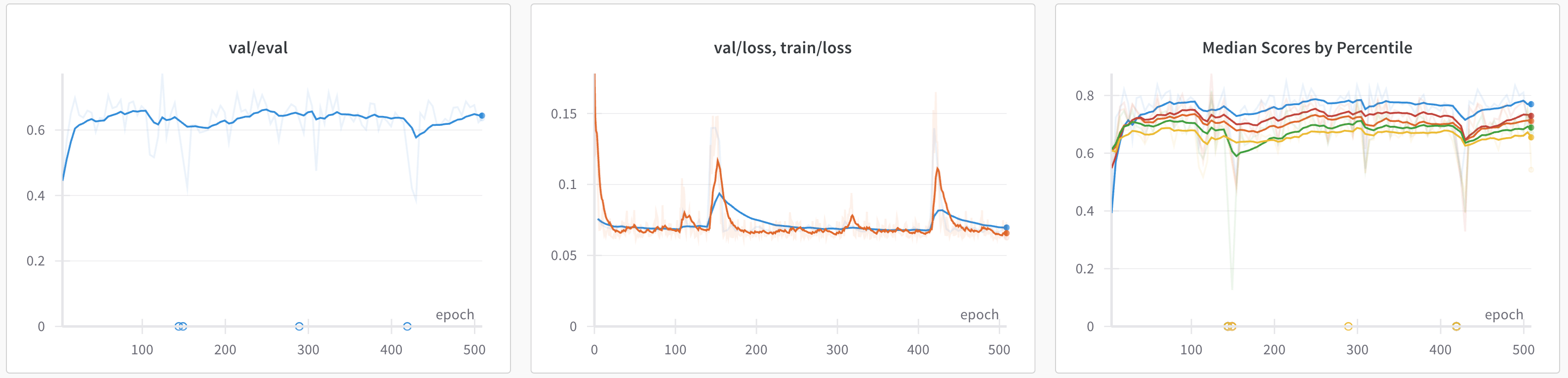
Although we have carefully designed an array of quantitative metrics, we do not simply deploy our best-performing models. Instead, we run a battery of qualitative analyses for our models. Generally, each model outputs some kind of artifact that represents inference on some relevant data. For example, we have a model that predicts fund performance and it outputs a list of funds with a predicted performance score over time. We have new data that we ingest daily into our systems, so we can run this model regularly to get new predictions. We have dashboards that report out these metrics for every training run that we have, a sample of which is shown below.

We have created a pipeline and testing yoke that not only allows us to analyze models on their own for our investment team, but it also allows us to run cross-model analyses using a potentially large set of model instances. In fact, we can produce hundreds of model candidates in a single sweep, so we can use our qualitative analysis pipeline to study the performance of all of these models at once.

Because of the results we see, both quantitative and qualitative, from our model analyses, we have started to work on ensembles of possibly very diverse models. Philosophically, this approach aligns with the general wisdom that a large collection of uncorrelated weak learners can become a strong learner.

Conclusion

We firmly believe in data-driven investment decisions. One of the more interesting aspects of working at Level is the diversity of data we work with, especially our dynamic graphs. While dynamic networks exist all around us, they are not a well-understood mathematical object and, indeed, we hope to stay at the forefront of modeling techniques for dynamic graphs. We hope that this brief exposition has given you a sense of the kind of work we do and the kind of problems we solve. If you’re interested in more details or to get into the technical weeds, please reach out to us!