Here at Level, we build a variety of statistical models. These models are predicting something that is inherently random. For example, if we are predicting the projected returns of a particular fund, our model may give us an estimate that, in expectation, the fund will have 5x returns over three years — a stellar result! However, this prediction is the average outcome and, given the nature of venture, many outcomes are highly volatile. Taking our previous example, how would feel if you knew that there's a 50% chance that its returns are flat (1x)?

To address these types of "distributional" concerns, we look at model predictions and their related confidence distributions. These confidence distributions can generate all sorts of ancillary information that help us quantify the amount of uncertainty in the model, the dataset, and the underlying thing we are trying to predict.

One technique we have recently deployed is the Jackknife. Jackknife and its updated version, Jackknife+, are powerful statistical techniques to estimate confidence for a set of predictions. Jackknife itself is old, introduced by Quenouille and Tukey (the great statistician and mathematician). Jackknife+ is an update to this method introduced by Barber, Candès, Ramdas, and Tibshirani in 2020.

The secret sauce of Jackknife+ is brilliantly simple: instead of training one model, we train a bunch of them. Each time we train one of these constituent models, we leave out a little bit of the data. That way, each constituent model has slightly different information from the rest of them; we can then measure how well each model does on that little bit that we left out and estimate how good each constituent model is. Finally, when we go to make a prediction on a unseen data, we generate a prediction from every constituent model and correct for its known error. This technique is statistically rigorous; the downside that it is computationally expensive, but we can easily parallelize Jackknife+, so it's possible for us to run it properly in practice.

The Math of Jackknife+

Let's suppose we have \( n \) data points in \( \mathbb{R}^{k} \) and and we are trying to predict a target scalar value. For a particular model \( \mu : \mathbb{R}^{k} \to \mathbb{R} \), we have to compute a full set of leave-one-out (LOO) predictions; for example, if we have \( 1 \, 000 \) data points, we have to train the model \( 1 \, 000 \) times, each time leaving out one data point.

For a particular data point \( i \in \{1, \ldots, n\} \subset \mathbb{N} \), our model is trying to minimize \( \mu(x_i) - y_i \), where \( x_i \) is the feature vector for data point \( i \) and \( y_i \) is its corresponding target value. We call this the residual for data point \( i \). In general, models try to minimize the residuals for all data points at once and different models make different trade-offs for different data points. However, we also want our model to generalize to new data, rather than simply memorizing it. The Jackknife+ method is a way to estimate the generalization error of a model.

To be precise, for Jackknife+, we have to do the following at training time:

1. Train models \( \mu_i \) on every point except the data point \( i \).
2. Compute the residual for each model on each point \( R_i \triangleq |\mu_i(x_i) - y_i| \).

Then, at inference time for new point \( x_{n+1} \), we can compute the Jackknife+ estimate by:

1. Computing the prediction for this new point under each model \( \mu_i(x_{n+1}) \).
2. Computing the lower residuals \( \mathcal{R}_{-} \triangleq \{\mu_i(x_{n+1}) - R_i\} \) and the upper residuals \( \mathcal{R}_{+} \triangleq \{\mu_i(x_{n+1}) + R_i\} \).
3. For confidence level \( \alpha \), compute \( v_{-} \) to be the \( \lfloor \alpha (n + 1) \rfloor \) smallest value in \( \mathcal{R}_{-} \) and compute \( v_{+} \) to be the \( \lceil (1 - \alpha) (n + 1) \rceil \) smallest value in \( \mathcal{R}_{+} \).
4. Return the interval \( [v_{-}, v_{+}] \) as the Jackknife+ confidence interval with confidence level \( 1 - \alpha \).

One thing to note here: the lower and upper residuals actually give us a full confidence distribution; if we wanted to change the confidence level or compute one-tailed confidence bounds, we do not need to do much work. We can compute any such questions from the lower and upper residuals.

Testing

We already use a traditional train–validate–test–predict split of our data for our modeling problems. One byproduct of this split is that we can actually go back and test that Jackknife+ works correctly. Although it is a theoretically sound model, it relies on some basic assumptions that do not always hold in the real world. We have to make sure that iff we generate a 80% confidence interval, it's confidence level is empirically 80%.

To test Jackknife+, we run it as we would normally. Then, we generate predictions in the test set, which is a set of data with known ground truth values, but are completely hidden from the training process. If we generate an 80% confidence interval from Jackknife+, then we would expect that 80% of the ground truth test set target values fall into their respective intervals.

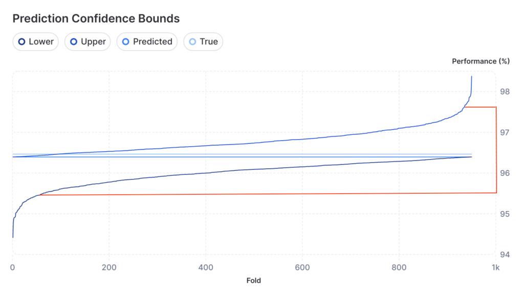
In practice, we tend to see about a 5–10% degradation in confidence levels, which means that if we want to generate an empirical 80% confidence interval, we actually need to set our theoretical confidence level to 85% or 90% to get the confidence that we need. This type of empirical degradation is normal and generally comes from three factors:

1. Data distributions shift. In statistical theory, you will often see these three letters: iid. This simple phrase makes us shudder in practice. For most theoretical results, we assume that all of our data is independent and identically distributed. Independence means that each data point is statistically unrelated to every other data point, which is simply just not true. Identically distributed means that all of our data comes from the same underlying distribution, but data distributions have a tendency to shift over time and, somewhat vexingly, seemingly at random. However, statistical theory is not useless: we instead need to be very careful, since we will inevitably break some of these assumptions. In addition to running various empirical tests to catch deviations from iid, we also deploy in-house technology to catch data drift issues.
2. It's hard to generate perfect train–validate–test splits of data. Again, there is a lot of theory behind how we should split our data, but, in practice, it's impossible to follow this theory perfectly. Inevitably, some of our test data will look a bit different from our train data; we run many analyses to help minimize this difference and, where possible, we account for it rigorously.
3. Everything is noisy. From data collection, to data reporting, to modeling, to analyses, to statistical tests: we are inherently dealing with fallible and random systems. While it's possible to eliminate noise, we use techniques like Jackknife+ to combat high-noise data to extract actionable insights.

Jackknife+ is not the only technique in Uncertainty Quantification (UQ) for modeling. As a firm, we have regular reading groups to stay on top of the technical literature. We're always looking out for the latest and greatest research ideas and we strive to iterate on these techniques quickly to see what will be useful to our modeling efforts.

P.S. if you read the Jackknife+ paper, we'll note that we technically use a variant of it called CV+, but it is largely the same idea with practical handling for large datasets.